Linear Regression with Gradient Descent Maths, Implementation and Example Using Scikit-Learn

We all know the famous Linear Regression algorithm, it is probably the oldest known algorithm in the world used in statistics and other fields. If you are not familiar with Linear Regression, check out this article first as it will help you in understanding the concepts of Linear Regression with Gradient Descent much better.

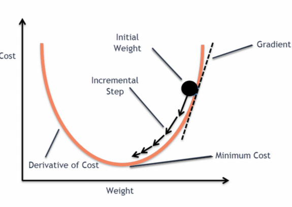
A gradient is an increase or decrease in the magnitude of the property(weights). In our case, as the gradient decreases our path becomes smoother. Gradient descent might seem like a terrifying concept but all it is doing is updating the weights and slope of the features in every single iteration.

Remember the equation for Linear Regression

#Linear Regression
Y=b0+b1*x
where b0 is the slope
b1 is the weight of independent feature x

Now there are a few additional equations you will have to know with Gradient Descent (i)Weight optimization and (ii)delta(error of the model).

#weight optimization for b0
w(t+1)=w(t)-alpha*delta
#weight optimization for b1
w(t+1)=w(t)-alpha*delta*x
where
w(t+1) is the new updated weight
w(t) is the old weight
alpha is the learning rate (0.1,0.001,0.0001)
delta is the error
#error
error=p(i)-y(i)
where p(i)= b0+b1*x
and y(i) is the dependent value of that iteration

The weight optimization for b0 and b1 is almost the same, except in b1 we multiply it with “x”, just like we do in linear regression. Recall in the last paragraph I said that we update the values of weight and slope in each iteration so, in the first iteration b0=0,b1=0 and learning rate will be 0.01.

X(independent)=[1,2,4,3,5] and Y(dependent)=[1,3,3,2,5]

#Iteration 1
b0(t)=0, b1(t)=0, x=1 and y(i)=1
#calculate p(i)
p(i)=b0+b1*x --> 0+0*1 --> 0
#calculate error
error=p(i)-y(i)-->0-1=-1
#calculate b0(t+1) new weight knowing that b0(t)=0
b0(t+1)=b0(t)-alpha*error --> 0-0.01*-1 ---> 0.01
#calculate b1(t+1) new weight knowing that b1(t)=0
b1(t+1)=b1(t)-alpha*error --> 0.-0.01*-1*1 --> 0.01

The newly updated weights are b0(t)=0.01 and b1(t)=0.01. We will use this weight for the next iteration where x=2 and y=3

#iteration 2
#calculate p(i)
p(i)=b0+b1*x --> 0.01+0.01*2 ---> 0.03
#calculate error
error=p(i)-y(i)--> 0.03-3 ---> -2.97
#calculate b0(t+2) knowing b0(t+1)
b0(t+2)=b0(t+1)-alpha*error --> 0.01-0.01*-2.97 ---> 0.0397
#calculate b1(t+2) knowing b1(t+1)
b1(t+2)=b1(t+1)-alpha*error*x --> 0.01-0.01*-2.97*2 ---> 0.0694
#iteration 3
x=4,y=3,b0(t+2)=0.0397,b1(t+2)=0.0694
p(i)=0.3173
error=-2.6827
b0(t+3)=0.066527
b1(t+3)=0.176708

We need to keep calculating the new slope and weights until we get the least residual when we plug b0 and b1 in Y=b0+b1*x. I hope you understood how the weights are updated as it is crucial to the working of the Gradient descent. Here is a python program to perform the same calculations.

z=1
for i,j in zip(x,y):
    if(z==1):
        b_0=0
        b_1=0
    if(z>=2):
        b_0=b_01
        b_1=b_11
        
    Y=b_0+b_1*i
    error=Y-j
    b_01=b_0-0.01*error
    b_11=b_1-0.01*error*i
    print(str(z)+"'st Iteration||||",'B0:',round(b_01,4),'||| B1:',round(b_11,4))
    z=z+1
##OUTPUT
1'st Iteration|||| B0: 0.01 ||| B1: 0.01
2'st Iteration|||| B0: 0.0397 ||| B1: 0.0694
3'st Iteration|||| B0: 0.0665 ||| B1: 0.1767
4'st Iteration|||| B0: 0.0806 ||| B1: 0.2188
5'st Iteration|||| B0: 0.1188 ||| B1: 0.4101

Just to check for our curiosity if updating the weights indeed gives us a more accurate prediction. We will plug in the second last row value from the data where x=3 and y=2.

#iteration 0
b0=0 and b1=1
Y=0+0*3 --> 0
#iteration 1
b0=0.01 and b1=0.01
Y=0.01+0.01*3 --> 0.04
#iteration 2
b0=0.0397
b1=0.0694
Y=0.0397+0.0694*3 --> 0.2479
#iteration 3
b0=0.066527
b1=0.176708
Y=0.066527+0.176708*3 --> 0.596651
#iteration 4
b0=0.0806
b1=0.2188
Y=0.0806+0.2188*3 --> 0.737
#iteration 5
b0=0.1188
b1=0.4101
Y=0.1188+0.4101*3 --> 1.3491

As you can see with each iteration the error in the prediction is decreasing and we are getting closer to the predicted value. If we continue this process for say 20 iterations, we will have a more precise prediction. We can apply the gradient descent algorithm using the scikit learn library. It provides us with SGDClassfier and SGDRegressor algorithms. Since this is a Linear Regression tutorial I will show you how to use SGDRegressor to make predictions. The dataset we will be using is the “Boston House Price Dataset”.

#importing libraries
from sklearn import linear_model 
from sklearn.datasets import load_boston
from sklearn.decomposition import PCA
from sklearn.preprocessing import StandardScaler
from sklearn.model_selection import cross_val_score
from sklearn.metrics import r2_score, mean_squared_error
from sklearn.pipeline import Pipeline
import numpy as np
import pandas as pd
#loading the data
X=load_boston()
data=pd.DataFrame(X.data,columns=X.feature_names)
Y=X.target
#Creating A Model
pipe=[]
pipe.append(('SC',StandardScaler()))
pipe.append(('PCA',PCA(n_components=8)))
pipe.append(('SGD',linear_model.SGDRegressor(alpha=0.1,learning_rate='adaptive',max_iter=300,penalty='elasticnet')))
model=Pipeline(pipe)
#cross validation score
cv_results = cross_val_score(model, data, Y, cv=5)
msg = "%s: %f (%f)" % ('SGDRegressor', cv_results.mean(), cv_results.std())
print(msg)
#output: 
SGDRegressor: 0.492394 (0.260191)
#Parameters to tune for SGDRegressor
params={
    'alpha':[0.1,0.01,0.001,0.0001,0.00001],
    'learning_rate':['constant','optimal','invscaling','adaptive'],
    'max_iter':[100,300,600,1000,1200,1500,2000],
    'penalty':['l2','l1','elasticnet']
}

According to the cross-validation score, we have an average mean of 0.492394 and average standard deviation of 0.260191. This is a satisfactory score but remember we didn't perform any of EDA methods on the data expect for PCA and feature Scaling using StandardScaler. There you have it guys, I have provided you with the basic information to get you started with SGDRegressor.

Please do give me feedback on how you liked this article. Also if you found any mistakes or think I can make some improvements to the article your opinion is welcome. Thank you for reading.

Links:

MachineLearningMastery:https://machinelearningmastery.com/implement-linear-regression-stochastic-gradient-descent-scratch-python/

Scikit-learn:https://scikit-learn.org/stable/modules/generated/sklearn.linear_model.SGDRegressor.html

Github:https://github.com/nitin689